ECODOPS - Efficient Coverage of Data On Parameter Space
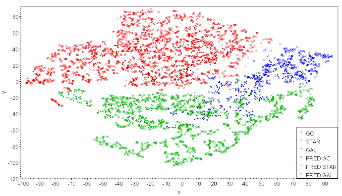
This page is the entry point to the ECODOPS software tool, specialized for data visualization through 2D maps able to inspect the coverage in the multidimensional feature space of the training and inference data. This is done by projecting the feature space onto two dimensions using the t-SNE method.
Release Notes
- Release currently available:
- Rel. 0.4 This is the last version, written in Python, running on a stable platform, compatible with Python 3.7.x or higher, deployed in February 2020.
Scope
In addition to optimizing the Parameter Space (PS), by selecting all relevant features, we need to make sure that in any classification experiment the training data cover the feature space sufficiently well for the classification in the inference data to result qualitatively acceptable.
Machine Learning (ML) models can be interpreted as complex decision boundaries in the training feature space. The models are expected to learn true patterns, which should then extend their applicability to new datasets. However, for the points that lie outside of the original region of feature space for which decision boundaries were created, model predictions may implement a classification function extrapolated from the training data, which may then not agree with the patterns outside of the training set. The most straightforward solution is to simply match the inference dataset to the training sample. Simple and commonly used solutions could consist into cutting data at some magnitude-limit, or, by working in the colour space, at some colour level.
Cuts performed in single features allow for a better match between the training and inference set in these particular dimensions. However, as the final classification is performed in a space of significantly larger dimensionality, the usefulness of such an approach can be rather limited. A match among individual features does not have to imply proper coverage of the full feature space. A simple counterexample is a 2D square covered by data points drawn from a 2D Gaussian distribution and separated into two subsets by a diagonal. In such case, the histograms of single features show overlap of data in individual dimensions, while in fact there is no data from two subsets overlapping in 2D at all. Therefore, we look in more detail at coverage in the multidimensional feature space of the training and inference data. This is done by projecting the feature space onto two dimensions using the t-SNE method.

There are many ways of mapping N-dimensional feature spaces onto 2D projections. A popular one in astronomy is Self Organizing Map (SOM, Kohonen 1997), and a relevant example of its usage is mapping of multi-color space to visualize which regions are not covered by spectroscopic redshifts (Masters et al. 2015). Here, we use another advanced visualization method, the t-distributed stochastic neighbor embedding (t-SNE, van der Maaten & Hinton 2008), which finds complex nonlinear structures and creates a projection onto an abstract low-dimensional space. Its biggest advantage over other methods is that t-SNE can be used on a feature space of even several thousand dimensions and still create a meaningful 2D embedding. Moreover, unlike in SOM where data points are mapped to cells gathering many observations each, in t-SNE every point from the N-dimensional feature space is represented as a single point of the low-dimensional projection. This makes t-SNE much more precise, allowing to plot the exact data point values over visualized points as different colors or shapes, making the algorithm output easier to interpret. Some disadvantages of using t-SNE are its relatively long computing time and its inability to map new sources added to a dataset after the transformation process, without running the algorithm again.
The t-SNE method makes use of the Kullback-Leibler (K-L) divergence cost function to find an optimal 2D representation of a multi-dimensional space. Through a cyclic process, the method tries to minimize the K-L divergence between the joint probabilities of the low-dimensional embedding and the high-dimensional data.
Documentation and Software
- ECODOPS User and Reference Manual
- Python software package
